Most people know that their chances of getting cancer increase as they age. In fact, by looking at data compiled by the National Cancer Institute, you can readily see that the incidence of cancer increases dramatically between the ages of 35 and 80.
A first-order ordinary differential equation
 " />
" />
has the solution
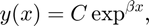 " />
" />
where  is any constant. This equation has infinitely many solutions depending on the coefficient .
However, this solution exhibits:
- exponential decay when
 and
and - exponential growth when

Could we use this simple first-order ordinary-differential equation to describe the increase in the cancer incidences with advancing age?
- Set-up
- Load the data
- The first order linear differential equation
- Set up basis functions for X
- Run Data2LD
- Plot the fitted curve with its confidence and prediction intervals
- Plot the estimated parameters of the ODE and their approximated CI with respect to rho
- Check fit to the ODE
- Check the residuals
- Check the normality
- Check the fitted vrs residuals plot
Set-up
clear
clear functions
close all
Load the data
load('Cancer_D.mat')

'ko');
set(phdl, 'LineWidth', 2)
xlabel('Age')
ylabel('Cancer cases per 100,000 population')
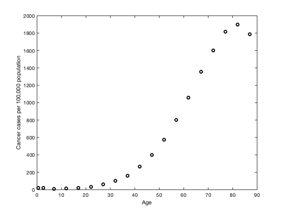
Figure (1) illustrates  observations of cancer cases measured from age 0.5 (6 months) to age 87.
The first order linear differential equation
The first order linear differential equation, as used in this example is
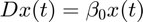 " />
" />
The parameter  in the linear ODE conveys the exponential growth (if positive) or decay (if negative) in the cancer cases per 100,000 population as the individuals increase in age.
Our aim is to estimate the cancer cases  and the parameter
  from the data in Figure (1).
Set up basis functions for X
rng = [yCell{1}(1,1),yCell{1}(end,1)];
knots = linspace(rng(1),rng(end),17);
norder = 4;
nbasis = length(knots)+ (norder - 2);
Xbasisobj = create_bspline_basis(rng,nbasis,norder,knots);
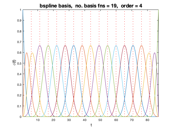
For the expansion of we used order four B-spline functions which by their nature have quadratic 1st derivatives. We used 17 equally spaced knots between the first age and last age.
Run Data2LD
...
estimate);
Elapsed time is 0.146885 seconds.
Rho = 0.017986
Elapsed time is 0.022159 seconds.
Iter. Criterion Grad Length
0 0.685044 2.899689
1 0.585193 0.006353
2 0.585192 0.000099
3 0.585192 0.000000
Convergence reached
Rho = 0.047426
Elapsed time is 0.007115 seconds.
Iter. Criterion Grad Length
0 2.157501 31.580614
1 0.986640 0.011659
2 0.986639 0.000000
3 0.986639 0.000000
Convergence reached
Rho = 0.1192
Elapsed time is 0.004404 seconds.
Iter. Criterion Grad Length
0 1.364304 15.111482
1 1.183677 0.120201
2 1.183659 0.007687
3 1.183659 0.000000
4 1.183659 0.000000
Convergence reached
Rho = 0.26894
Elapsed time is 0.004613 seconds.
Iter. Criterion Grad Length
0 2.210732 5.826973
1 2.206174 2.003834
2 2.205552 0.000007
3 2.205552 0.000007
Convergence reached
Rho = 0.5
Elapsed time is 0.005504 seconds.
Iter. Criterion Grad Length
0 8.932094 24.668212
1 8.927238 19.587081
2 8.918894 0.001299
3 8.918894 0.001299
Convergence reached
Rho = 0.73106
Elapsed time is 0.007391 seconds.
Iter. Criterion Grad Length
0 50.086004 317.404345
1 49.902561 211.418297
2 49.753985 0.020389
3 49.753985 0.000003
Convergence reached
Rho = 0.8808
Elapsed time is 0.004991 seconds.
Iter. Criterion Grad Length
0 273.304443 3492.861116
1 266.798749 830.525108
2 266.392399 0.247578
3 266.392399 0.000023
4 266.392399 0.000023
Convergence reached
Rho = 0.95257
Elapsed time is 0.008163 seconds.
Iter. Criterion Grad Length
0 1287.717764 25966.624253
1 1208.446766 11.389006
2 1208.446749 0.052566
3 1208.446749 0.052566
Convergence reached
Rho = 0.97069
Elapsed time is 0.004982 seconds.
Iter. Criterion Grad Length
0 2428.563193 31142.857569
1 2368.963070 3.445830
2 2368.963069 0.006817
3 2368.963069 0.006817
Convergence reached
Rho = 0.98201
Elapsed time is 0.004668 seconds.
Iter. Criterion Grad Length
0 4489.782266 64097.659926
1 4354.083523 726.414294
2 4354.065327 2.028102
3 4354.065327 0.000001
4 4354.065327 0.000001
Convergence reached
Rho = 0.98901
Elapsed time is 0.006144 seconds.
Iter. Criterion Grad Length
0 7722.533872 120190.917904
1 7449.157831 5617.334077
2 7448.539950 19.824171
3 7448.539942 0.000162
4 7448.539942 0.000162
Convergence reached
Rho = 0.99331
Elapsed time is 0.004972 seconds.
Iter. Criterion Grad Length
0 12251.252245 206960.235730
1 11762.237808 3729.638910
2 11762.077813 9.427963
3 11762.077812 0.000010
4 11762.077812 0.000010
Convergence reached
Rho = 0.99593
Elapsed time is 0.004120 seconds.
Iter. Criterion Grad Length
0 17729.824401 324423.391751
1 16999.609058 9741.163187
2 16998.958673 2.315216
3 16998.958673 2.315216
Convergence reached
Rho = 0.99753
Elapsed time is 0.006425 seconds.
Iter. Criterion Grad Length
0 23218.776058 436232.145878
1 22415.648247 38845.867141
2 22409.253363 31.166360
3 22409.253359 0.000294
4 22409.253359 0.000294
Convergence reached
Rho = 0.9985
Elapsed time is 0.004287 seconds.
Iter. Criterion Grad Length
0 27807.849171 471685.381726
1 27181.928628 46.098778
2 27181.928622 0.046046
3 27181.928622 0.046046
Convergence reached
Rho = 0.99909
Elapsed time is 0.004165 seconds.
Iter. Criterion Grad Length
0 31251.304301 415132.875069
1 30889.361861 25.389049
2 30889.361859 0.008810
3 30889.361859 0.008810
Convergence reached
Rho = 0.99945
Elapsed time is 0.004520 seconds.
Iter. Criterion Grad Length
0 33695.515579 315771.647591
1 33521.806820 2.157681
2 33521.806820 2.157681
Convergence reached
Rho = 0.99966
Elapsed time is 0.004981 seconds.
Iter. Criterion Grad Length
0 35358.129071 219301.132475
1 35283.440727 0.766985
2 35283.440727 0.766985
Convergence reached
Rho = 0.9998
Elapsed time is 0.004569 seconds.
Iter. Criterion Grad Length
0 36448.866477 144230.172265
1 36418.736938 0.276752
2 36418.736938 0.276752
Convergence reached
Rho = 0.99988
Elapsed time is 0.005201 seconds.
Iter. Criterion Grad Length
0 37145.107063 91831.001853
1 37133.429812 4772.896008
2 37133.397841 0.049178
3 37133.397841 0.049178
Convergence reached
Rho = 0.99993
Elapsed time is 0.004548 seconds.
Iter. Criterion Grad Length
0 37581.254238 57349.299817
1 37576.805174 1356.638427
2 37576.802667 0.006333
3 37576.802667 0.006333
Convergence reached
Rho = 0.99995
Elapsed time is 0.006344 seconds.
Iter. Criterion Grad Length
0 37851.149662 35402.716121
1 37849.479451 352.401304
2 37849.479285 0.000678
3 37849.479285 0.000678
Convergence reached
Elapsed time is 0.054914 seconds.
Optimal rho values:
Rho Theta1 sdTheta1 MSE ISE Df GCV
_____ ______ ________ _____ _____ _____ _____
1 0.037 0.004 37577 0.026 1.116 42415
All rho values:
Rho Theta1 sdTheta1 MSE ISE Df GCV
_____ ______ ________ ______ ______ ______ ______
0.018 0.154 0.12 0.585 291.41 18.156 296.72
0.047 -0.038 0.16 0.987 171.35 18.064 406.38
0.119 -0.011 0.084 1.184 172.45 18.015 440.22
0.269 -0.009 0.042 2.206 361.52 17.944 714.28
0.5 -0.008 0.028 8.919 638.99 17.652 1772
0.731 -0.006 0.02 49.754 841.37 16.611 3146.7
0.881 -0.002 0.014 266.39 817.49 14.284 4324.1
0.953 0.004 0.01 1208.4 600.26 11.043 6890.9
0.971 0.008 0.009 2369 461.15 9.396 9271.9
0.982 0.012 0.008 4354.1 324.9 7.867 12682
0.989 0.017 0.008 7448.5 205.69 6.504 17219
0.993 0.022 0.007 11762 114.04 5.316 22677
0.996 0.026 0.006 16999 54.728 4.294 28374
0.998 0.03 0.005 22409 23.403 3.426 33351
0.998 0.033 0.005 27182 9.363 2.714 36998
0.999 0.034 0.004 30889 3.621 2.164 39339
0.999 0.035 0.004 33522 1.374 1.763 40731
1 0.036 0.004 35283 0.516 1.488 41532
1 0.036 0.004 36419 0.192 1.306 41992
1 0.037 0.004 37133 0.071 1.189 42258
1 0.037 0.004 37577 0.026 1.116 42415
1 0.037 0.004 37849 0.01 1.071 42507
The GCV indicates a model with a lower  provides a model with better predictive power. This suggests that the differential equation does not describe the behaviour of the data well and perhaps a more complex equation would provide a better description of the data.
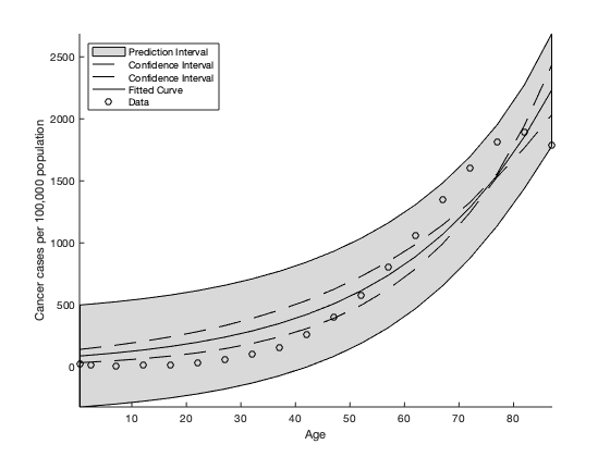
Plot the fitted curve with its confidence and prediction intervals
This Figure illustrates the cancer cases per 100,000 population indicated by the circles. The fitted curve produced by Data2LD with  (solid line), the approximated 95% pointwise confidence interval for the curve (dashed line) and the approximated 95% pointwise prediction interval for the curve (grey region).
t seems the differential equation is too simple to capture the behaviour of the cancer cases; maybe we should try letting the parameter  vary over age. This implies that the rate of growth/decline of cancer incidences changes with advancing age. See for the analysis with an age-varying parameter for further details.
figure(4)
hp = patch([yCell{1}(:,1); yCell{1}(end:-1:1,1);yCell{1}(1)],...
    [Results_cell{4}(:,4); Results_cell{4}(end:-1:1,5); Results_cell{4}(1)],[0.85 0.85 0.85]);
hold on;
plot(yCell{1}(:,1),[Results_cell{4}(:,2),Results_cell{4}(:,3)],'k--')
plot(yCell{1}(:,1),Results_cell{4}(:,1),'k-')
plot(yCell{1}(:,1), yCell{1}(:,2), 'ko');
xlim([min(yCell{1}(:,1))-0.1,max(yCell{1}(:,1))+0.1])
ylim([min(Results_cell{4}(:,4))-0.1,max(Results_cell{4}(:,5))+0.1])
xlabel('Age')
ylabel('Cancer cases per 100,000 population')
legend('Prediction Interval','Confidence Interval','Confidence Interval','Fitted Curve','Data','Location','northwest')
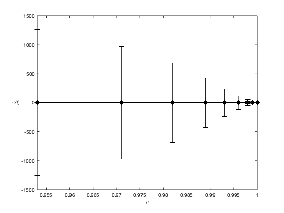
Plot the estimated parameters of the ODE and their approximated CI with respect to rho
The values of the parameter and its approximated 95% confidence interval over values of converging to 1.0. Note the reduction in the width of the approximated 95% confidence intervals as increase and the overlap of the final estimates of the ODE parameter, which illustrates that the parameter value has stabilised for high values of .
The optimal estimate of the parameter is  with a 95% confidence interval between 0.028 and 0.045.
Res_Mat         = table2array(Res);
df              = Results_cell{3,1}(3);
t_v             = tinv(0.975,length(yCell{1}(:,1))-df);
indexOfInterest = (Res_Mat(:,1) > 0.95);

figure(5)
plot(Res_Mat(indexOfInterest,1),Res_Mat(indexOfInterest,2),'-*k')
hold on;
errorbar(Res_Mat(indexOfInterest,1),Res_Mat(indexOfInterest,2),...
    t_v.*Res_Mat(indexOfInterest,5),'ko')
xlabel('$rho
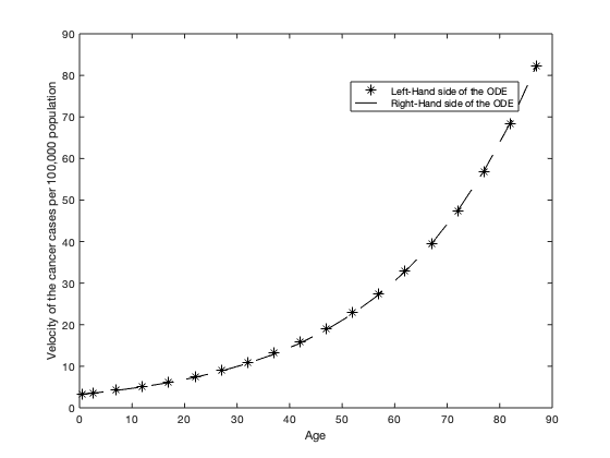
Check fit to the ODE
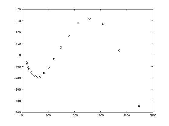
Dfit   = eval_fd(yCell{1}(:,1), getfd(Results_cell{1}),1);
RHS    = Results_cell{2}(1).*Results_cell{4}(:,1);

figure()
plot(yCell{1}(:,1),Dfit,'*k')
hold on;
plot(yCell{1}(:,1),RHS,'k--')
legend('Left-Hand side of the ODE','Right-Hand side of the ODE','Location','best')
xlabel('Age')
ylabel('Velocity of the cancer cases per 100,000 population')
The difference between the LHS and RHS of the ODE is negligible, indicating that the ODE is satisfied.
Check the residuals
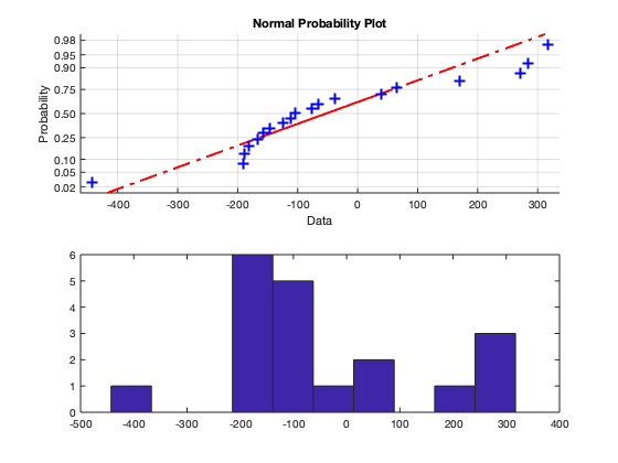
Check the normality
res = yCell{1}(:,2)-Results_cell{4}(:,1);
figure()
subplot(2,1,1)
h = normplot(res);
h(1).LineWidth = 2;
h(2).LineWidth = 2;
h(3).LineWidth = 2;
subplot(2,1,2)
hist(res)
Our qqplot indicates that the residuals are not normal distribution, as the quantiles of the residuals do not generally line up with the red dashed line. The histogram does not have the features of a normal distribution. That is it's not symmetric and does not have a bell-shape.
Check the fitted vrs residuals plot
figure()
plot(Results_cell{4}(:,1),yCell{1}(:,2)-Results_cell{4}(:,1),'ko')
If the model is specified correctly, we should see random scatter in a constant band around zero with no patterns in the plot and no funnels. We can see a clear non-linear pattern in the below plot indicating that the model does not adequately capture the complexity of the data.